Nesting algorithm

Nesting Algorithms are used to make the most effecient use of material or space by evaluating many different possible combinations via Recursion.

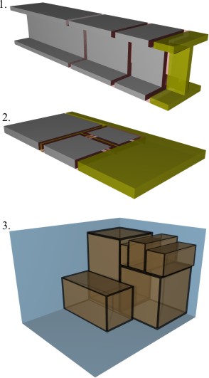
1. Linear (1-dimensional)

The simplest of the algorithms illustrated here.

For an existing set there is only one position where a new cut can be placed--at the end of the last cut.

Validation of a combination involves a simple Stock - Yield - Kerf = Scrap calculation.
2. Plate (2-dimensional)

These algorithms are significantly more complex.

For an existing set, there may be as many as eight positions where a new cut may be introduced next to each existing cut, and if the new cut is not perfectly square then different rotations may need to be checked.

Validation of a potential combination involves checking for intersections between two-dimensional objects.
3. Packing (3-dimensional)

These algorithms are the most complex illustrated here due to the larger number of possible combinations.

Validation of a potential combination involves checking for intersections between three-dimensional objects.

Linear (1-dimensional) cut combinations:

Plate (2-dimensional) cut combinations:

Kerf
Area, shape, and useability of resulting scrap or drop
Cost or preference of source material
Number of cuts required
Density (Yield Area / Cut Bounding Box)
i.e. If a combination consists of only two rectangular 1x2' cuts, placing them parallel results in a higher density than placing them in a T or L shape.